The Inelastic Hard Rods model
We introduce a system of hard rods (the length of the rods ![]() is
not relevant, as already discussed in paragraph
3.1.1), confined to a ring and colliding
inelastically. Two rods collide if and only if they are at contact and
their relative velocity is of opposite sign with respect to the
relative position, i.e.
is
not relevant, as already discussed in paragraph
3.1.1), confined to a ring and colliding
inelastically. Two rods collide if and only if they are at contact and
their relative velocity is of opposite sign with respect to the
relative position, i.e.
![]() .
.
After a binary collision the scalar velocities of the particles change according to:
where ![]() is the restitution coefficient, which takes the value
is the restitution coefficient, which takes the value ![]() for perfectly elastic systems and 0 for completely inelastic
particles (in this case,
for perfectly elastic systems and 0 for completely inelastic
particles (in this case, ![]() , equivalent to the sticky gas model).
Few years ago McNamara and Young [158], and Sela and
Goldhirsch [197], simulated such a model and observed a
universal algebraic decay of the kinetic energy,
, equivalent to the sticky gas model).
Few years ago McNamara and Young [158], and Sela and
Goldhirsch [197], simulated such a model and observed a
universal algebraic decay of the kinetic energy,
![]() (Haff's Law [103]), together with an anomalous behavior for
the global velocity distribution, even in the early homogeneous
regime. Furthermore, strong inhomogeneities appeared as the precursor
of a numerically catastrophic event, the inelastic collapse: particles
perform an infinite number of collisions in finite time interval [157].
(Haff's Law [103]), together with an anomalous behavior for
the global velocity distribution, even in the early homogeneous
regime. Furthermore, strong inhomogeneities appeared as the precursor
of a numerically catastrophic event, the inelastic collapse: particles
perform an infinite number of collisions in finite time interval [157].
As already discussed, the renewal of interest on one-dimensional
granular flows, has been generated by the recent work of Ben-Naim et
al [22]. They have circumvented the inconvenience of the
inelastic collapse, by means of a sort of ``regularization'': they
assumed that when two particles collide with an absolute relative
velocity lesser than an arbitrary cut-off
![]() , the
collision occurs elastically. This is not too
different from the proposed visco-elastic model (see paragraph
2.1.5), where the restitution coefficient depends on the
relative velocity of the colliding objects. Moreover, the authors have
verified that the main results (e.g. the asymptotic energy decay) do
not depend on the choice of the cut-off
, the
collision occurs elastically. This is not too
different from the proposed visco-elastic model (see paragraph
2.1.5), where the restitution coefficient depends on the
relative velocity of the colliding objects. Moreover, the authors have
verified that the main results (e.g. the asymptotic energy decay) do
not depend on the choice of the cut-off ![]() . Furtherly, we have
checked that these (and other) results can be reproduced using the
visco-elastic regularization, and they are quite independent from the
details of the functional form
. Furtherly, we have
checked that these (and other) results can be reproduced using the
visco-elastic regularization, and they are quite independent from the
details of the functional form
![]() . The choice of
regularization, i.e. of the value of
. The choice of
regularization, i.e. of the value of ![]() , of course is relevant
for the length of the simulation: the system in fact behaves mostly as
an elastic gas when a large part of the molecules have reached a
velocity of the order of
, of course is relevant
for the length of the simulation: the system in fact behaves mostly as
an elastic gas when a large part of the molecules have reached a
velocity of the order of ![]() . This quasi-elastic final
stage is
. This quasi-elastic final
stage is ![]() -dependent.
-dependent.
However this regularizations allows the system to enter into a
dynamical regime which was not investigated in the past (many authors,
to prevent the collapse, chose smaller systems, but this prevented
also the long wavelength instabilities). As discussed before, during
such a regime, the kinetic energy decays as
![]() ,
for any
,
for any ![]() . A direct inspection of the hydrodynamic profiles,
shows that such a regime is highly inhomogeneous, with density
clusters and shocks in the velocity field. Accordingly, they suggest
that inelastic systems behave asymptotically as a sticky (
. A direct inspection of the hydrodynamic profiles,
shows that such a regime is highly inhomogeneous, with density
clusters and shocks in the velocity field. Accordingly, they suggest
that inelastic systems behave asymptotically as a sticky (![]() )
gas [57] which is known to be described by the Burgers
equation in the inviscid limit [199]. Such a behavior
reflects the fact that the asymptotics is dominated by the dynamics of
clusters of particles, which move through the system and coalesce,
similarly to sticky objects. As already pointed out, one of the main
predictions of the Burgers conjecture is the
)
gas [57] which is known to be described by the Burgers
equation in the inviscid limit [199]. Such a behavior
reflects the fact that the asymptotics is dominated by the dynamics of
clusters of particles, which move through the system and coalesce,
similarly to sticky objects. As already pointed out, one of the main
predictions of the Burgers conjecture is the
![]() scaling distribution, which could not be verified
in the work of Ben-Naim and co-workers.
scaling distribution, which could not be verified
in the work of Ben-Naim and co-workers.
The 1d Inelastic Lattice Gas model
Alternatively, one may attack the Boltzmann equation, by assuming a
simpler form for the scattering cross section in the collision
integral, i.e. taking the relative velocity of the colliding pair to
be proportional to the average thermal velocity:
![]() . This is the so called pseudo-Maxwell model [33],
discussed in detail in paragraph 5.1.5.
. This is the so called pseudo-Maxwell model [33],
discussed in detail in paragraph 5.1.5.
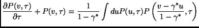
The energy factor ![]() can be eliminated via a time
reparametrization, and one obtains a simpler equation:
can be eliminated via a time
reparametrization, and one obtains a simpler equation:
where
![]() and the
and the ![]() counts the number of collisions
per particle. Eq. (5.40) is the master equation of the
inelastic version of Ulam's scalar model: at each step an
arbitrary pair is selected and the scalar velocities are transformed
according to the rule of Eq. (5.39).
counts the number of collisions
per particle. Eq. (5.40) is the master equation of the
inelastic version of Ulam's scalar model: at each step an
arbitrary pair is selected and the scalar velocities are transformed
according to the rule of Eq. (5.39).
This model accounts for mean field behavior, i.e. disregards spatial
correlation. Therefore it cannot give reliable results in the
correlated phase that one expects after the end of the Homogeneous
Cooling. Moreover, it does not reproduce the behavior of the Hard Rod
model even in the homogeneous phase, as it is demonstrated in the next
section (this in general means that the so-called ``homogeneous''
phase is not really homogeneous, even if it is characterized by a
Haff-like decay of the energy which, in ![]() is found only in a
non-correlated system). To reinstate spatial correlation we considered
the
is found only in a
non-correlated system). To reinstate spatial correlation we considered
the ![]() version of the Inelastic Lattice Gas model introduced in the
previous section.
version of the Inelastic Lattice Gas model introduced in the
previous section. ![]() sites disposed on a line with periodic boundary
conditions have associated a ``velocity''
sites disposed on a line with periodic boundary
conditions have associated a ``velocity'' ![]() . At every step of the
evolution a pair of neighboring sites is chosen randomly and undergoes
an inelastic collision according to Eq.(5.39) if
. At every step of the
evolution a pair of neighboring sites is chosen randomly and undergoes
an inelastic collision according to Eq.(5.39) if
![]() . The latter condition, which avoids
collisions between particles ``moving'' far from each other, is to be
be referred below as the kinematic constraint and plays a key
role in the formation of structures during the inhomogeneous phase. A
unit of time
. The latter condition, which avoids
collisions between particles ``moving'' far from each other, is to be
be referred below as the kinematic constraint and plays a key
role in the formation of structures during the inhomogeneous phase. A
unit of time ![]() correspond to
correspond to ![]() collisions (i.e. to
collisions (i.e. to ![]() collision per particle on average).
collision per particle on average).