When an instability arises, structures emerge. The characterization of structures is achieved by means of correlation functions or structure factors (their Fourier transforms):
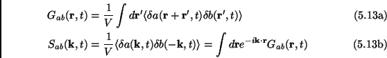 |
where ![]() is the volume of the system.
is the volume of the system.
If the quantities ![]() and
and ![]() in the above formulas are components
in the above formulas are components ![]() and
and ![]() of a vector
of a vector
![]() (e.g. the components
(e.g. the components ![]() and
and ![]() of the
velocity vector
of the
velocity vector
![]() ), then the functions
), then the functions ![]() and
and
![]() become isotropic tensor and can be decomposed in two scalar
isotropic functions:
become isotropic tensor and can be decomposed in two scalar
isotropic functions:
 |
It is immediate to verify that, if the vector
![]() is
decomposed into
is
decomposed into ![]() components
components ![]() perpendicular to
perpendicular to
![]() and one component
and one component
![]() parallel to
parallel to
![]() ,
then
,
then
 |
or, if
![]() is decomposed into
is decomposed into ![]() components
components ![]() perpendicular to
perpendicular to
![]() and one component
and one component
![]() parallel
to
parallel
to
![]() , then
, then
 |
We use in the rest of this section the subscript ![]() and
and
![]() to indicate the structure factors and correlation
functions relative to the velocity vector decomposed in parallel and
perpendicular components, i.e.
to indicate the structure factors and correlation
functions relative to the velocity vector decomposed in parallel and
perpendicular components, i.e.
![]() .
.
In the isotropic tensor case (the one defined just above) it is often convenient to subtract the self-correlation equilibrium part from the correlation function and from the structure factor, i.e. defining:
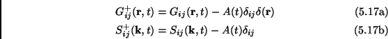 |
where
![]() , e.g. if
, e.g. if
![]() then
then
![]() .
.
The further assumption of incompressibility (which plays an important
role in the following), states that
![]() or, equivalently:
or, equivalently:
 |
(5.19) |
The study of correlation functions in cooling granular gases has been
carried along by several authors. In particular the group of van Noije
and co-workers has developed two lines of reasoning: a study of the
ring kinetic theory [210] and a study of fluctuating
hydrodynamics [212]. The first can be considered more
fundamental, as it copes with kinetic degrees of freedom, while the
second is based on the hydrodynamics description of the fluctuations,
and therefore is less general.
Correlation functions from ring kinetic theory
The correlation function is directly related to the the pair
correlation function
![]() (discussed in paragraph
2.2.7), by the relation:
(discussed in paragraph
2.2.7), by the relation:

The authors [210] have calculated, using the second of the ring kinetic equations 2.96, the structure factor for the correlation of shear mode fluctuations:
with
![]() is the same
correlation length appearing in the dispersion relations of the
previous paragraph. This expression for the structure factor is
identical to the energy spectrum
is the same
correlation length appearing in the dispersion relations of the
previous paragraph. This expression for the structure factor is
identical to the energy spectrum ![]() in the theory of
in the theory of ![]() or
or ![]() homogeneous turbulence in incompressible fluids.
homogeneous turbulence in incompressible fluids.
The expression for the correlation functions indicates that
![]() . The authors
have performed 2D molecular dynamics simulations at low solid
fraction (
. The authors
have performed 2D molecular dynamics simulations at low solid
fraction (![]() ) obtaining a good verification of their
results.
) obtaining a good verification of their
results.
Correlation functions from fluctuating hydrodynamics
At the hydrodynamic level (
![]() ) the correlation functions and
structure factors can be obtained from the so-called fluctuating
hydrodynamics [137]. This method consists in the study of
coupled linear Langevin equations for the values of the hydrodynamic
fields, obtained considering the linear transport of linearized
hydrodynamics equation as the systematic (dissipative) part of the
equations, while the noise is given by fluctuations of fluxes
(momentum and heat):
) the correlation functions and
structure factors can be obtained from the so-called fluctuating
hydrodynamics [137]. This method consists in the study of
coupled linear Langevin equations for the values of the hydrodynamic
fields, obtained considering the linear transport of linearized
hydrodynamics equation as the systematic (dissipative) part of the
equations, while the noise is given by fluctuations of fluxes
(momentum and heat):
 |
(5.21) |
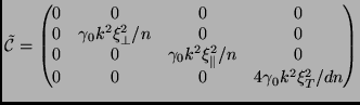
where the vector
![]() and the matrix
and the matrix
![]() have been defined in the previous paragraph. The
noise
have been defined in the previous paragraph. The
noise
![]() is given by internal fluctuations of the
fluxes. The fluxes (or currents)
is given by internal fluctuations of the
fluxes. The fluxes (or currents)
![]() and
and
![]() are
considered fluctuating around their average values:
are
considered fluctuating around their average values:
 |
where the fluctuating part of the currents is assumed to be a white Gaussian noise, local in space, with correlations given by appropriate fluctuation-dissipation relations (they can be found on the last chapter of [137]):
 |
(with ![]() the bulk viscosity, defined in paragraph
2.3.9) so that the (derived)
fluctuation-dissipation relations for the noise
the bulk viscosity, defined in paragraph
2.3.9) so that the (derived)
fluctuation-dissipation relations for the noise
![]() are given by:
are given by:
 |
(5.24) |
with
(as it can be seen, different components of noise are uncorrelated, and in the equation for the density there is no noise).
The results of the analysis is reviewed in the following table:
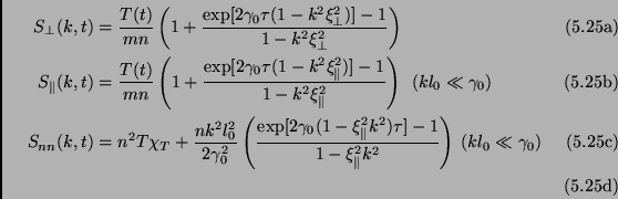 |
The structure factor for the shear modes is identical to that derived
from the ring kinetic equations (Eq. (5.22)). The factors
calculated for the longitudinal velocity components and for the
density fluctuations are obtained in the dissipative range
(
![]() ), in the absence of propagating modes (all
eigenvalues of the linear stability matrix are real).
), in the absence of propagating modes (all
eigenvalues of the linear stability matrix are real).
The above expressions for the structure factors yields the following important conclusions:
Incompressible and compressible flows
An important assumption can be used to simplify the study of structures in cooling granular gases, that of incompressibility. This is a fairly realistic assumption for what concerns ordinary elastic fluids, so we can consider it applicable also to granular gases for small inelasticity.
In terms of hydrodynamics fields, it states that
![]() , and in terms of fluctuations modes it implies that
, and in terms of fluctuations modes it implies that
![]() . The consequence of this is that
. The consequence of this is that
![]() , that the density structure factor
, that the density structure factor ![]() does not evolve in time and that the temperature fluctuations
does not evolve in time and that the temperature fluctuations
![]() simply decay as kinetic modes, staying spatially
homogeneous. With this assumption is also easier to calculate the
spatial correlation functions
simply decay as kinetic modes, staying spatially
homogeneous. With this assumption is also easier to calculate the
spatial correlation functions
![]() . It has been found
that these correlation functions exhibits power law tails
. It has been found
that these correlation functions exhibits power law tails
![]() [212].
[212].
Moreover there is a difference between the two correlation functions:
![]() has a negative minimum in correspondence with
has a negative minimum in correspondence with ![]() (this
can be identified as the mean diameter of vortices), while
(this
can be identified as the mean diameter of vortices), while
![]() is always positive.
is always positive.
If the incompressibility assumption is relaxed (this is necessary at
high inelasticity), the behavior of the correlation functions at
large ![]() changes. It happens that an exponential cut-off superimposes
over the power law tail
changes. It happens that an exponential cut-off superimposes
over the power law tail ![]() , at a typical distance
, at a typical distance
![]() . The power law behavior becomes an intermediate
behavior, observable if
. The power law behavior becomes an intermediate
behavior, observable if
![]() and
and ![]() are well
separated. In the compressible regime [213], the correlation
function of the density fluctuations shows a typical length scale
are well
separated. In the compressible regime [213], the correlation
function of the density fluctuations shows a typical length scale
![]() which agrees with the prediction of the structure factor.
which agrees with the prediction of the structure factor.
![$\displaystyle S_\perp^+(k,t)=\frac{T(t)}{mn} \frac{\exp [2 \gamma_0 \tau(1-k^2 \xi_\perp^2) ]-1}{1-k^2\xi_\perp^2}$](img1453.png)