The most complicated of the transport equations presented above is
that for the general heat flow
![]() . This set of
. This set of ![]() scalar
quantities are tied to the fourth order corrections in the
Chapman-Enskog expansion (see (2.135)). In most physical
problems it is usually sufficient to know the evolution of the
contracted quantity
scalar
quantities are tied to the fourth order corrections in the
Chapman-Enskog expansion (see (2.135)). In most physical
problems it is usually sufficient to know the evolution of the
contracted quantity
![]() defined in Eq. (2.119),
which represents the transport of the total (modulus) random energy of
the particles due to the random motion of the molecules (we lose
accuracy on the transport of single random velocity
components). Therefore we make the assumption:
defined in Eq. (2.119),
which represents the transport of the total (modulus) random energy of
the particles due to the random motion of the molecules (we lose
accuracy on the transport of single random velocity
components). Therefore we make the assumption:
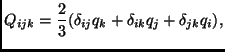
reducing the set of ![]() components to only
components to only ![]() contracted components.
contracted components.
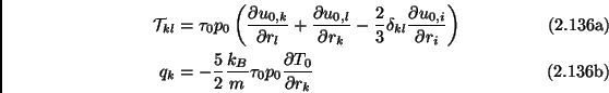
With this further assumption it is more easy to perform the BGK calculation of the collision terms that appear in the stress and heat tensor equations (2.138). Bypassing the details the final formula are:
 |
(2.135) | |
| (2.136) |
This last result is very important if inserted in equations
(2.138). In fact it must be noted that the
second and third order expansion coefficients (ultimately tied to
![]() and
and
![]() ) are usually negligibly small, except
when they are multiplied by very large factors, in this case
) are usually negligibly small, except
when they are multiplied by very large factors, in this case
![]() . The Chapman-Enskog method can only be applied to gases
which are not far from equilibrium: this means that very frequent
collisions must nearly absorb all deviations from equilibrium. In
other words the relaxation time
. The Chapman-Enskog method can only be applied to gases
which are not far from equilibrium: this means that very frequent
collisions must nearly absorb all deviations from equilibrium. In
other words the relaxation time ![]() must be extremely
short. Based on this argument, we can neglect all terms containing the
stress tensor and the heat flow vector, except the ones which are
multiplied by
must be extremely
short. Based on this argument, we can neglect all terms containing the
stress tensor and the heat flow vector, except the ones which are
multiplied by ![]() , obtaining (for the case
, obtaining (for the case
![]() ):
):
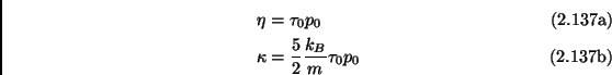
which is the familiar linear relation between the flows and the gradients: momentum flow (non-diagonal) is proportional to the velocity gradient, heat flow is proportional to temperature gradient. Having recognized that, the hydrodynamic transport coefficients (viscosity and heat conductivity) can be expressed:
that are equivalent (with slight differences in the numerical constants) with the mean free path calculations discussed in paragraph 2.1.4.
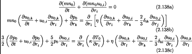
The ![]() Navier-Stokes equations can be finally obtained:
Navier-Stokes equations can be finally obtained:
These equations represent the most simple form of transport equations for a gas that is not in strict local thermodynamic equilibrium (which instead is described by Euler equations (2.123)). The deviation from equilibrium is slight but important, as irreversible (dissipative) processes emerge from it: these are taken into account by the linear transport coefficients (viscosity and heat conductivity) which represent the tendency of the gas to relax toward the Maxwellian equilibrium.