The phase space distribution function and its moments

We assume that a phase space distribution function can be defined:

$$N(t,\mathbf{r},\mathbf{v})=P(t,\mathbf{r},\mathbf{v})d^3r d^3v$$ (2.101)

where $N(t,\mathbf{r},\mathbf{v})$ is the number of particles found at time $t$ near the point $\mathbf{r},\mathbf{v}$ of the phase space. $P$ is assumed to be the solution of the Boltzmann Equation (2.74).

The particle number density is defined as

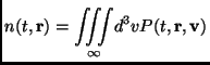$$n(t,\mathbf{r})=\underset{\infty}{\iiint}d^3vP(t,\mathbf{r},\mathbf{v})$$ (2.102)

The average molecular velocity is defined as

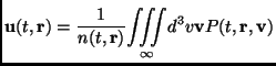$$\mathbf{u}(t,\mathbf{r})=\frac{1}{n(t,\mathbf{r})}\underset{\infty}{\iiint}d^3v \mathbf{v}P(t,\mathbf{r},\mathbf{v})$$ (2.103)

and this allows to introduce the random velocity vector

$$\mathbf{c}(t,\mathbf{r})=\mathbf{v}-\mathbf{u}(t,\mathbf{r})$$ (2.104)

which depends on time and position (while $\mathbf{v}$ is independent of $t$ and $\mathbf{r}$) and has zero average:

$$\underset{\infty}{\iiint}d^3cc_iP(t,\mathbf{r},\mathbf{c})=0$$ (2.105)

The average fluxes of the molecular quantity $W(\mathbf{v})$ can be expressed as velocity moments of the phase space distribution function:

$$j_W^i(t,\mathbf{r})=\underset{\infty}{\iiint}d^3vv_iW(\mathbf{v})P(t,\mathbf{r},\mathbf{v})$$ (2.106)

When $W=m$ one has the mass flux:

$$j_m^i=mn(t,\mathbf{r})u_i(t,\mathbf{r}).$$ (2.107)

When $W=mv_j$ one has the momentum flux:

$$j_{mv_j}^i=mn(t,\mathbf{r}) \langle v_i v_j \rangle=mnu_iu_j+mn \langle c_i c_j \rangle$$ (2.108)

which is a $3 \times 3$ symmetric matrix. In the last form two contributions can be recognized, that is the flux due to the bulk (organized) motion and the flux resulting from the random (thermal) motion of the gas particles. This second term is usually called the pressure tensor $\mathcal{P}_{ij}=mn \langle c_i c_j \rangle$. One can define, from this discussion, two quantities that are the scalar pressure $p$ and the vector temperature $T_i$:

$$p = \frac{1}{3}(\mathcal{P}_{xx}+\mathcal{P}_{yy}+\mathcal{P}_{zz})$$ (2.109)

$$\frac{1}{2}k_BT_i = \frac{1}{2}m \langle c_i^2 \rangle= \frac{1}{2}\frac{\mathcal{P}_{ii}}{n}$$ (2.110)

and in the isotropic case $T_i=T$ so that $p=nk_BT$. It can be also defined the stress tensor $\mathcal{T}$ as:

$$\mathcal{T}_{ij}=\delta_{ij}p-\mathcal{P}_{ij}$$ (2.111)

which expresses the deviation of the pressure tensor from the equilibrium Maxwellian case (for which $\mathcal{P}_{ij}=p\delta_{ij}$).

Finally, the flux of the quantity $W=mv_jv_k$ is given by:

$$j_{mv_jv_k}^i=mnu_iu_ju_k+u_i\mathcal{P}_{jk}+u_j\mathcal{P}_{ik}+u_k\mathcal{P}_{ij}+\mathcal{Q}_{ijk}$$ (2.112)

where $\mathcal{Q}_{ijk}=mn \langle c_i c_j c_k \rangle$ is the generalized heat flow tensor and describes the transport of random energy $c_j c_k$ due to thermal motion $c_i$ of the molecules (for all the permutations of $i,j,k$).

In equation (2.118) three contributions can be recognized: the first term describes the bulk transport of the bulk flux of momentum; the second, third and fourth terms describe the a combination of bulk and random momentum fluxes; the last term is the transport of random energy component due to the random motion itself. Often a ``classical'' heat flow vector is introduced, more intuitive than the generalized heat flow tensor:

$$q_i=\frac{\mathcal{Q}_{ikk}}{2}=n \left \langle c_i \frac{mc^2}{2} \right \rangle.$$ (2.113)

It is also of use to give the definition of the fourth velocity moment:

$$\mathcal{R}_{ijkl}(t,\mathbf{r})=mn \langle c_i c_j c_k c_l \rangle$$ (2.114)