Elementary transport calculations

In the kinetic theory the condition of equilibrium is equivalent to the absence of macroscopic flows, i.e. absence of transport. The transport of the molecular quantity $W$ along a particular direction $\hat{\mathbf{n}}$ is characterized by its net flux $\mathbf{j}_W(t,\mathbf{r}) \cdot \hat{\mathbf{n}}$ which is defined as the net fraction of $W$ crossing in the unit time a unit surface normal to the direction $\hat{n}$ in the point $\mathbf{r}$ of the space. If the quantity $W$ is always transported by molecular motion or transferred from a particle to another via collision interactions that conserve the sum of $W$ (i.e. $W$ is said to be a collisional invariant), then the variation in time of the coarse grained field $W(t,\mathbf{r})$ (which is an average of $W$ taken on particles in a well suited region of space-time centered in $(t,\mathbf{r})$) is simply expressed by a continuity formula:

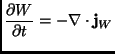$$\frac{\partial W}{\partial t}= -\nabla \cdot \mathbf{j}_W$$ (2.35)

In elastic gases the relevant conserved molecular quantities are: $m$, $m \mathbf{v}$ and $mv^2/2$, that is mass, momentum and energy.

Empirical observations show that, in situations not too far from equilibrium almost all the transport fluxes are proportional to the spatial gradient of the transported quantity:

$$\mathbf{j}_W=-C_W\nabla W$$ (2.36)

where $C_W$ is called the transport coefficient for the quantity $W$. The most important transport coefficients are: the diffusion coefficient $D$ (transport of mass or self diffusion), the viscosity $\eta$ (transport of transversal momentum, e.g. transport of $mv_x$ in the direction $y$ or $z$) and the heat conductivity $\kappa$ (transport of heat, that is internal energy). The flux of longitudinal momentum (e.g. $mv_x$ in the direction $x$) is somewhat different as it is dominated by an order zero (in the spatial gradients) contribution which is given by the hydrostatic pressure $p$ (in the Boltzmann-Grad limit $p=nk_BT$).

Starting from the basic concepts of mean free time and path, it is possible to derive heuristic expressions for the transport coefficients [62]. Such calculations, that take the name of mean free path method are meaningful in the limit of small Knudsen numbers:

$$=\frac{\lambda}{L} \ll 1$$ (2.37)

where $\lambda$ is the mean free path and $L$ is the characteristic linear size of the problem (related to boundary conditions, e.g. in a shear experiment $L=\overline{v}/\gamma$ where $\overline{v}$ is the thermal velocity of the fluid and $\gamma=\Delta u_x/\Delta L_y$ is the shear rate). This condition corresponds to the necessity that the variation of all macroscopic quantities is small within a mean free path.

With this assumption, very rough calculations carry to good estimates of the main transport coefficients:

In the last formulas the rightmost sides are calculated using the expressions for the mean free path and for the average velocity modulus obtained with the assumption of Maxwell-Boltzmann equilibrium. In the above equations one sees that the viscosity and the heat conductivity do not depend on the density, but only on the temperature of the gas. Apparently one expects that the viscosity depends upon the density (more particles carry more momentum) but in these approximated calculations the fluxes are assumed to be carried only by molecular motion (i.e. collisional transfer is negligible): for the viscosity for example this means the appearance of the product $n \lambda$ which does not depend on $n$ (as $\lambda$ is inversely proportional to $n$).