The Inelastic Lattice Gas model

The model that we introduce is a lattice gas with constant density. It is constituted by the association of a d-dimensional velocity field $\mathbf{v}_i$ with every node of a d-dimensional lattice of linear extension $L$. $N$ is the number of nodes in the lattice. The density of the ``fluid'' is considered constant and homogeneous throughout the whole system. In this way the dynamics of the gas consists of collisional events only. Hereafter we report the study performed in two dimensions on a triangular lattice [11,14]. In the next chapter we will study the lattice in $d=1$. We adopt periodic boundary conditions, so that finite size effects emerge if and only if the correlation lengths grow up to the size of the lattice, otherwise the system can be considered ``without borders''.

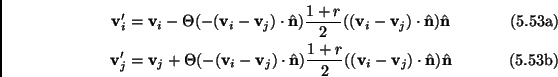
At each step of the dynamics a nearest neighbor pair of nodes $(i,j)$ is randomly selected and the two velocities are updated according to the rule:

where $\hat{\mathbf{n}}=(\mathbf{r}_i-\mathbf{r}_j)/\vert(\mathbf{r}_i-\mathbf{r}_j)\vert$ represents the unit vector pointing from site ${\bf j}$ to ${\bf i}$, $\Theta$ is the Heaviside step function and $r \in [0,1]$ is the normal restitution coefficient. We measure the time $\tau$ using the non dimensional number of collisions per particle, i.e. a time interval $\Delta \tau=1$ represents $N$ collisions. In each inelastic collision (Eq.(5.57)) the total linear and angular momentum are conserved, whereas a fraction $\vert(\mathbf{v}_i-\mathbf{v}_j)\cdot \hat{\mathbf{n}}\vert^2(1-r^2)/4$ of the relative kinetic energy is dissipated. The inelasticity of the collisions has the effect of reducing the quantity $\vert({\bf v_i-v_j}) \cdot \hat{\mathbf{n}}\vert$, inducing a partial alignment of the velocities. The presence of the $\Theta$ enforces the kinematic constraint that plays an important role in the development of structures, as shown below.

We note that when the velocity vectors are totally uncorrelated with each other, the evolution of the single-site probability $P(\mathbf{v},t)$ should obey some kind of closed master equation similar to the Boltzmann equation. It is important to stress that in the dynamics proposed here, there is no dependence of the scattering cross section (or the collision rate) upon the relative velocity of the colliding sites. This means that the master equation should resemble the Boltzmann equation for the pseudo-Maxwell model introduced in the previous section (see paragraph 5.1.5).

Another consideration must be done, in order to make interesting connections with other fields of the physics of systems out of equilibrium. The cooling process exhibits striking similarities with the quench of a magnetic system from an initially stable disordered phase at a temperature $T_0$ to an ordered phase at a lower temperature $T_{quench}$. In a standard quench process [38] one usually considers the process by which a thermodynamic system, brought out of equilibrium by a sudden change of an external constraint, such as temperature or pressure, finds its new equilibrium state: this means that the typical processes of phase ordering (expected after the quench) happen while the external temperature is constant (often equal to zero). In the cooling of a granular fluid one wants to study the relaxation of a fluidized state after the external driving force (whose role is to reinject the energy dissipated by the collisions, keeping the system in a statistically steady state) is switched-off abruptly at some time $\tau=0$. Due to the competition of different configurations with comparable dissipation rates, the system does not relax immediately toward a motionless state, but displays a complex phenomenology similar to that observed in a coarsening process.

A last remark concerns the term incompressibility, which cannot be used rigorously in our model. In fact the continuity equation

$$\frac{\partial n}{\partial t}=\frac{\partial (n u_i)}{\partial r_i}$$ (5.55)

states that if the density is constant in space and time, then

$$\frac{\partial u_i}{\partial r_i} \equiv 0$$ (5.56)

And this is equivalent, in Fourier space, to the equation

$$\mathbf{k} \cdot \mathbf{u} \equiv 0$$ (5.57)

i.e.: there are no longitudinal velocity fluctuations, and therefore the correspondent structure factor vanishes, $S_\parallel \equiv 0$. This does not happen in our model, as the velocity is here only a passive mode, i.e. there is no coupling with the density (which actually does not exist). Longitudinal fluctuations can be present even if the fluid has constant density. Of course, we can consider our model as quasi-incompressible, i.e.: the longitudinal fluctuations of the velocity field are present but are much less important than the transverse fluctuations, so that the density transport can be neglected.