The binary collision operator
![]() , for inelastic
particles, must be changed [210] according to the inelastic collision rules,
Eqs. (2.41) and Eqs. (2.42). It must be
noted that when
, for inelastic
particles, must be changed [210] according to the inelastic collision rules,
Eqs. (2.41) and Eqs. (2.42). It must be
noted that when ![]() (elastic collisions), the two set of equations
coincide, i.e. the direct or inverse collision are identical
transformation. This is not true if
(elastic collisions), the two set of equations
coincide, i.e. the direct or inverse collision are identical
transformation. This is not true if ![]() . Therefore, in the
definition of the inverse binary collision operators at the end of
section 2.2.1, that is
. Therefore, in the
definition of the inverse binary collision operators at the end of
section 2.2.1, that is ![]() and
and
![]() , we have put the same operator
, we have put the same operator ![]() that
appears in the direct binary collision operators
that
appears in the direct binary collision operators ![]() and
and
![]() , while in general it must be used the operator
, while in general it must be used the operator
![]() that replaces velocities with precollisional velocities (using
the transformation given in Eqs. (2.42)). The adjoint of
inverse binary inelastic collision operator(the only one needed in the
following) therefore reads:
that replaces velocities with precollisional velocities (using
the transformation given in Eqs. (2.42)). The adjoint of
inverse binary inelastic collision operator(the only one needed in the
following) therefore reads:
![$\displaystyle \overline{T}_-(1,2)=\sigma^2\int_{\mathbf{V}_{12} \cdot \hat{\mat...
...thbf{n}})b_c'-\delta(\mathbf{r}_1-\mathbf{r}_2+\sigma\hat{\mathbf{n}}) \right ]$](img673.png) |
(2.94) |
Deriving from this the BBGKY hierarchy (analogue of (2.94)) and putting in the first equation of it the Molecular Chaos assumption, the Boltzmann Equation for granular gases is obtained [41,210]:
where the primed velocities are defined in Eqs. (2.42).
This equation has been studied in the spatially homogeneous case (no
spatial gradients, ![]() ), with the Enskog correction (i.e. a
multiplying factor
), with the Enskog correction (i.e. a
multiplying factor
![]() in front of the collision integral)
by Goldshtein and Shapiro [97] and by Ernst and van Noije [211]. The equation is
in front of the collision integral)
by Goldshtein and Shapiro [97] and by Ernst and van Noije [211]. The equation is
where
![]() . Goldshtein and Shapiro [97] have shown that
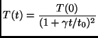
this equation admits an isotropic scaling solution which describes the
so-called ``Homogeneous Cooling State'', depending on time only
through the temperature
. Goldshtein and Shapiro [97] have shown that
this equation admits an isotropic scaling solution which describes the
so-called ``Homogeneous Cooling State'', depending on time only
through the temperature ![]() defined by the relation
defined by the relation
![]() :
:
with ![]() defined by the relation
defined by the relation
![]() .
.
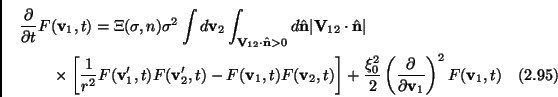
The scaling function solves a complicated integro-differential equation. This can be studied using an expansion in Sonine polynomials:
| (2.96) |
where
![]() ,
,
![]() is the Maxwellian
and
is the Maxwellian
and
![]() is the second Sonyne polynomial. The
calculations of Ernst and van Noije [211] have shown that for
is the second Sonyne polynomial. The
calculations of Ernst and van Noije [211] have shown that for
![]() the coefficient
the coefficient ![]() is very near to zero, precisely
is very near to zero, precisely
![]() in three dimensions and
in three dimensions and
![]() in two
dimensions. The decay of the temperature has also been calculated:
in two
dimensions. The decay of the temperature has also been calculated:
 |
(2.97) |
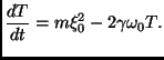
with
![]() (dimensionless damping rate),
(dimensionless damping rate),
![]() , and the initial Maxwellian mean free time
, and the initial Maxwellian mean free time
![]() (
(
![]() is the collision frequency
calculated with a Maxwellian with temperature
is the collision frequency
calculated with a Maxwellian with temperature ![]() ), while the true
collision frequency reads
), while the true
collision frequency reads
![]() . Monte
Carlo simulations (DSMC, see Appendix A) by Brey et al. [42] of the
Eq. (2.99) have shown that
the temperature decay and the fourth cumulant
. Monte
Carlo simulations (DSMC, see Appendix A) by Brey et al. [42] of the
Eq. (2.99) have shown that
the temperature decay and the fourth cumulant ![]() qualitatively
agree with the results of Ernst and van Noije. Moreover the agreement
between very dilute Molecular Dynamics simulations and Monte Carlo
solutions of the Boltzmann equation in 2D have shown
agreement up to moderate inelasticities (
qualitatively
agree with the results of Ernst and van Noije. Moreover the agreement
between very dilute Molecular Dynamics simulations and Monte Carlo
solutions of the Boltzmann equation in 2D have shown
agreement up to moderate inelasticities (
![]() ).
).
Ernst and van Noije [211] have also given estimates for the tails of the velocity distribution, using an asymptotic method employed by Krook and Wu [129]. This method assumes that for a fast particle the dominant contributions to the collision integral come from collisions with thermal (bulk) particles and that the gain term of the integral can be neglected with respect to the loss term. They found an exponential behavior for the tails of the scaling distribution function of velocities:
| (2.98) |
with ![]() a constant depending on
a constant depending on ![]() .
.
It is relevant that Ernst and van Noije have also studied Enskog-Boltzmann equation in the presence of a random forcing, i.e. a source of energy that acts randomly, uncorrelated and isotropically on all the particles. The homogeneous equation for this system reads:
where the velocity diffusion coefficient ![]() appears, which is
proportional to the rate of energy input per unit mass
appears, which is
proportional to the rate of energy input per unit mass
![]() . This equation admits a stationary homogeneous solution
. This equation admits a stationary homogeneous solution
![]() with
with ![]() defined as
above in terms of the granular temperature
defined as
above in terms of the granular temperature ![]() . It is immediate to
obtain a temperature balance
. It is immediate to
obtain a temperature balance
From Eq. (2.105)
follows the value for the stationary temperature (if the system
remains homogeneous!). The authors have also given estimates for the
coefficient ![]() of the Sonine expansion. Molecular dynamics by van
Noije et al. [211] have shown that the predictions of the homogeneous
Boltzmann equation work for
of the Sonine expansion. Molecular dynamics by van
Noije et al. [211] have shown that the predictions of the homogeneous
Boltzmann equation work for
![]() and low densities. The
Krook and Wu method for the asymptotic behavior of the tails of the
velocity distribution.function gives
and low densities. The
Krook and Wu method for the asymptotic behavior of the tails of the
velocity distribution.function gives
| (2.100) |
![\begin{multline}
\left( \frac{\partial}{\partial t}+L_1^0 \right)P(\mathbf{r}_1,...
...athbf{r}_1,\mathbf{v}_1,t)P(\mathbf{r}_1,\mathbf{v}_2,t) \right ]
\end{multline}](img674.png)
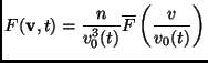
![\begin{multline}
\frac{\partial}{\partial t}F(\mathbf{v}_1,t) = \Xi(\sigma,n)\si...
...,t)F(\mathbf{v}_2',t)-F(\mathbf{v}_1,t)F(\mathbf{v}_2,t) \right ]
\end{multline}](img676.png)