In order to discuss the behavior of a system of ![]() identical hard
spheres (of diameter
identical hard
spheres (of diameter ![]() and mass
and mass ![]() ) it is natural to introduce
the phase space, i.e., a
) it is natural to introduce
the phase space, i.e., a ![]() dimensional space where the
coordinates are the
dimensional space where the
coordinates are the ![]() components of the
components of the ![]() position vectors of the
sphere centers
position vectors of the
sphere centers
![]() and the
and the ![]() components of the
components of the ![]() velocities
velocities
![]() . The state of the system is represented by a
point in this space. We call
. The state of the system is represented by a
point in this space. We call
![]() the
the ![]() -dimensional
position vector of this point. If the positions
-dimensional
position vector of this point. If the positions
![]() of the spheres are restricted in a space region
of the spheres are restricted in a space region
![]() , then the full phase space is given by the product
, then the full phase space is given by the product
![]()
If the state is not known with absolute accuracy, we must introduce a
probability density ![]() which is defined by
which is defined by
 |
(2.45) |
where
![]() is the Lebesgue measure in phase space and we implicitly
assume that the probability is a measure absolutely continuous with
respect to the Lebesgue measure.
is the Lebesgue measure in phase space and we implicitly
assume that the probability is a measure absolutely continuous with
respect to the Lebesgue measure.
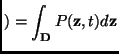
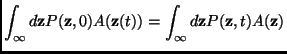
The mean value of a dynamical observable
![]() can be
calculated from either the following expressions:
can be
calculated from either the following expressions:
which are respectively the Lagrangian and Eulerian averages (analogous
to the Heisemberg and Schroedinger averages in quantum mechanics). In
Eq. (2.47) the time dependence of the observable ![]() and of
the distribution
and of
the distribution ![]() is due to the time evolution operator
is due to the time evolution operator ![]() (also
called streaming operator, that is
(also
called streaming operator, that is
![]() . Considering the equivalence in
Eq. (2.47) as an inner product implies that
. Considering the equivalence in
Eq. (2.47) as an inner product implies that
where
![]() is the adjoint of
is the adjoint of ![]() .
.
In a general system (not necessarily made of hard spheres) with
conservative and additive interactions, the force between the
particle pair ![]() is
is
![]() so that the time evolution operator is given by:
so that the time evolution operator is given by:
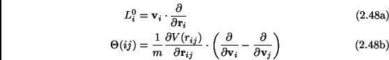
where the Liouville operator
![]() is
the Poisson bracket with the Hamiltonian, so that
is
the Poisson bracket with the Hamiltonian, so that
 |
and
![]() is a unitary operator,
is a unitary operator,
![]() ,
while
,
while
![]() . In Eq. (2.49) the evolution operator
. In Eq. (2.49) the evolution operator
![]() has been divided into a free streaming operator
has been divided into a free streaming operator
![]() which generates the free particle trajectories, plus a term
containing the binary interactions among the particles.
which generates the free particle trajectories, plus a term
containing the binary interactions among the particles.
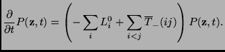
Finally the Liouville equation is obtained writing explicitly Eq. (2.48):
which is an expression of the incompressibility of the flow in phase space.
In the specific case of identical hard spheres, the interaction among particles is defined by Eq. (2.30). It can be shown that this kind of interaction carries no contraction of phase space at collision, i.e.
where
![]() and
and
![]() are the phase space points before
and after a collision. This can be considered a form of detailed
balance law. It is important to stress that
are the phase space points before
and after a collision. This can be considered a form of detailed
balance law. It is important to stress that
![]() : a collision represents a time discontinuity in the
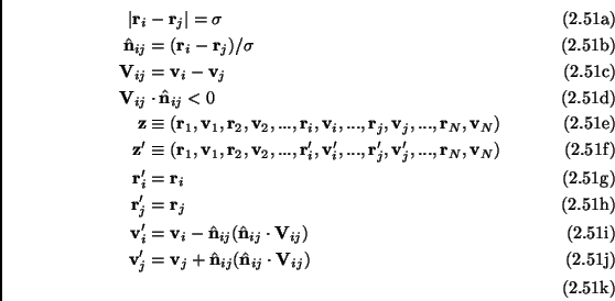
velocity section of phase space. In particular we use the elastic
collision model defined in this list of prescriptions (it coincides
with the collision rule for smooth hard spheres, see
Eq. (2.33)):
: a collision represents a time discontinuity in the
velocity section of phase space. In particular we use the elastic
collision model defined in this list of prescriptions (it coincides
with the collision rule for smooth hard spheres, see
Eq. (2.33)):
these relations conserve the total momentum and the total energy of the system.
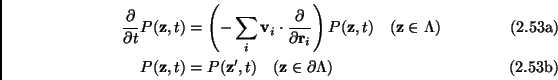
To derive the Boltzmann equation, the collisions events
![]() are
considered as boundary conditions and the Liouville Equation
(2.51) is restricted to the interior of the phase space
region
are
considered as boundary conditions and the Liouville Equation
(2.51) is restricted to the interior of the phase space
region
![]() where
where
| (2.53) |
is the set of phase space points such that one or more pairs of spheres are overlapping. With this conditions, the Liouville equation reads:
This version of the Liouville equation is time-discontinuous: this means that formal perturbation expansions used in usual many-body theory methods cannot be applied to it.
An alternative master equation for the probability density function in
the phase space can be derived [83]. The streaming operator ![]() for hard
spheres is not defined for any point of the phase space
for hard
spheres is not defined for any point of the phase space
![]() . In the calculation of the average
(2.47) of physical observables, this is not a problem, as
the streaming operators appears multiplied by
. In the calculation of the average
(2.47) of physical observables, this is not a problem, as
the streaming operators appears multiplied by
![]() which
is proportional to the characteristic function
which
is proportional to the characteristic function
![]() of the
set
of the
set ![]() (the characteristic function is
(the characteristic function is ![]() for points belonging
to the set and 0 for points outside of it). In perturbation
expansions it is safer to have a streaming operator defined for every
point of the configurational space. A standard representation, defined
for all points in the phase space, has been developed for elastic hard
spheres and is based on the binary collision expansion of
for points belonging
to the set and 0 for points outside of it). In perturbation
expansions it is safer to have a streaming operator defined for every
point of the configurational space. A standard representation, defined
for all points in the phase space, has been developed for elastic hard
spheres and is based on the binary collision expansion of
![]() in terms of binary collision operators. The binary
collision operator is defined in terms of two-body dynamics through
the following representation of the streaming operator for the
evolution of two particles:
in terms of binary collision operators. The binary
collision operator is defined in terms of two-body dynamics through
the following representation of the streaming operator for the
evolution of two particles:
with
![]() the free flow operator and a collision operator
the free flow operator and a collision operator
 |
(2.56) |
where ![]() is a substitution operator that replaces
is a substitution operator that replaces
![]() with
with
![]() (see
Eqs. (2.53)).
(see
Eqs. (2.53)).
The Eq. (2.56) is a representation of the
evolution of two particles as a convolution of free flow and
collisional events. Noting that
![]() for
for
![]() (two hard spheres cannot collide more than once),
Eq. (2.56) can be put in the form
(two hard spheres cannot collide more than once),
Eq. (2.56) can be put in the form
that can be generalized to the N-particle streaming operator (here considered for the case of an infinite volume):
where
 |
(2.59) |
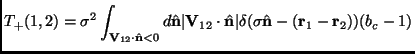
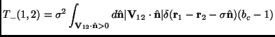
Equation (2.59) defines the so-called pseudo-streaming operator. In order to write an analogue of the
Liouville Equation (2.51), the adjoint of ![]() is
needed: its definition is identical to that in
Eq. (2.59) but for the binary collision operators
which must be replaced by their adjoints:
is
needed: its definition is identical to that in
Eq. (2.59) but for the binary collision operators
which must be replaced by their adjoints:
![$\displaystyle \overline{T}_\pm(1,2)=\sigma^2\int_{\mathbf{V}_{12} \cdot \hat{\m...
...a\hat{\mathbf{n}})b_c-\delta(\mathbf{r}_1-\mathbf{r}_2+\sigma\hat{\mathbf{n}})]$](img512.png) |
(2.60) |
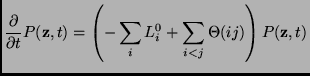
Finally the pseudo-Liouville equation can be written:
This equation is the analogue of Eq. (2.51) for the case of hard core potential (hard spheres). In this sense it replaces Eq. (2.55) and will be used in the following, precisely in paragraph 2.2.7, to derive kinetic equations different from the ones discussed just below.
![$\displaystyle S_t(\mathbf{z})=\exp[tL(\mathbf{z})]=\exp\left[ t \sum_iL_i^0-t\sum_{i<j}\Theta(ij) \right]$](img481.png)
![$\displaystyle S_{\pm t}(\mathbf{z})=\exp \left\{\pm t[L_0(\mathbf{z}) \pm \sum_{i<j}T_\pm (i,j)]\right\}$](img509.png)