Collision invariants, H-theorem and hydrodynamical limit

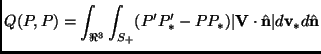
The integral appearing in the right-hand side of Eq. (2.74) is usually called collision integral:

$$Q(P,P)=\int_{\Re^3}\int_{S_+} (P'P_*'-PP_*)\vert\mathbf{V} \cdot \hat{\mathbf{n}}\vert d\mathbf{v}_*d\hat{\mathbf{n}}$$ (2.73)

where we have used an intuitive contracted notation (the prime or $*$ must be considered applied to the velocity vector in the argument of the function $P$). In the collision integral, the position $\mathbf{r}$ is the same wherever the function $P$ appears, and therefore it can be considered a parameter of $Q(P,P)$.

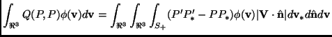
Let us have a look to the integral

$$\int_{\Re^3}Q(P,P)\phi(\mathbf{v})d\mathbf{v}=\int_{\Re^3}\int_{\... ...mathbf{V} \cdot \hat{\mathbf{n}}\vert d\mathbf{v}_*d\hat{\mathbf{n}}d\mathbf{v}$$ (2.74)

which can be transformed in many alternative forms, using its symmetries. In particular one can exchange primed and unprimed quantities, as well as starred and unstarred quantities. With manipulations of this sort, it is immediate to get the following alternative form of Eq. (2.77):

$$\int_{\Re^3}Q(P,P)\phi(\mathbf{v})d\mathbf{v} =\frac{1}{8}\int_{\... ...\hat{\mathbf{n}}\vert d\mathbf{v}_*d\hat{\mathbf{n}}\phi(\mathbf{v})d\mathbf{v}$$ (2.75)

From this equation it comes that if

$$\phi+\phi_*=\phi'+\phi_*'$$ (2.76)

almost everywhere in velocity space, then the integral of Eq. (2.78) is zero independent of the particular function $P$. Many authors have proved under different assumptions that the most general solution of Eq. (2.79) is given by

$$\phi(\mathbf{v})=C_1+ \mathbf{C}_2 \cdot \mathbf{v}+C_3\vert\mathbf{v}\vert^2$$ (2.77)

Furtherly, if $\phi=\log P$, from Eq. (2.78) it follows that

$$\int_{\Re^3}Q(P,P)\phi(\mathbf{v})d\mathbf{v} =\frac{1}{8}\int_{\... ...athbf{n}}\vert d\mathbf{v}_*d\hat{\mathbf{n}}\phi(\mathbf{v})d\mathbf{v} \leq 0$$ (2.78)

which follows from the elementary inequality $(z-y)\log(y/z) \leq 0$ if $y,z \in \Re^+$. This becomes an equality if and only if $y=z$, therefore the equality sign holds in Eq. (2.81) if and only if

$$P'P_*'=PP_*$$ (2.79)

This is equivalent to two important facts:

• $\phi+\phi_*=\phi'+\phi_*'$ (taking the logarithms of both sides of Eq. (2.82)), so that we can use the result (2.80) obtaining $P=\exp(C_1+C_2 \cdot \mathbf{v}+C_3\vert\mathbf{v}\vert^2)=C_0 \exp(-\beta\vert\mathbf{v}-\mathbf{v}_0\vert^2)$ where we have defined $C_0=\exp(C_1)$, $\beta=-C_3$ and $\mathbf{v}_0=\mathbf{C}_2/2\beta$; this function is called Maxwell-Boltzmann distribution or simply Maxwellian;

• $Q(P,P) \equiv 0$, i.e. the collision integral identically vanishes.

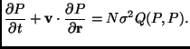
Equation (2.81) is a fundamental result of the Boltzmann theory (it is often called Boltzmann Inequality) and can be fully appreciated with the following discussion: we rewrite the Boltzmann Equation (2.74) with a simplified notation:

$$\frac{\partial P}{\partial t}+\mathbf{v} \cdot \frac{\partial P}{\partial \mathbf{r}}= N\sigma^2 Q(P,P).$$ (2.80)

We multiply both sides by $\phi=\log P$ and integrate with respect to $\mathbf{v}$, obtaining a transport equation for the quantity $\phi$:

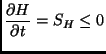
Then Eq. (2.81) states that $S_H \leq 0$ and $S_H =0$ if and only if $P$ is a Maxwellian. For example, if we look for a space homogeneous solution of the Boltzmann equation, it happens that

$$\frac{\partial H}{\partial t}=S_H \leq 0$$ (2.82)

that is the famous H-Theorem. It simply states that there exists a macroscopic quantity ($H$ in this case) that decreases as the gas evolves in time and eventually goes to zero when (if and only if) the distribution $P$ becomes a Maxwellian. When the homogeneity is not achievable (due to non-homogeneous boundary conditions) rigorous results are more complicated, but we are still tempted to say that the Maxwellian represents the local asymptotic equilibrium, with the spatial dependence carried by the parameters of this distribution function.

The H-Theorem shows that the Boltzmann equation, apparently obtained from microscopic reversible principles, has a basic feature of irreversibility: the trajectories in the phase space that corresponds to evolutions of the one-particle probability distribution that give place to an increase of $H$ with time are not solutions of the Boltzmann equation, even if they are compatible with the given collision rules, i.e. with the laws of Newtonian mechanics. This paradox [207,142] is nowadays discussed in the following way [61]: the assumption of Molecular Chaos is the source of irreversibility, the choice of factorization of probability for molecules that go into a collision induces correlations for the molecules that go out of a collision. If the velocity of all the molecules would be inverted at a certain time, the one particle probability distribution would no more satisfy the Molecular Chaos hypothesis and the Boltzmann equation could not describe the system. In general ``no kind of irreversibility cam follow by correct mathematics from the analytical dynamics of a conservative system'' (Cercignani et al. [61]). The other paradox often cited as a consequence of the H-Theorem is the so-called Zermelo's paradox [180,227]: Zermelo noted that the ``recurrence theorem'' of Poincare [179] is in contrast with the H-Theorem. The recurrence theorem guarantees that the molecules of the gas, after a ``recurrence time'', can have positions and velocities so close to the initial ones that the one particle distribution would be practically the same, that is if it decreased initially, then it must have increased ad some later time. The answer of Boltzmann [35] to this objection is that the recurrence time is so large that, practically speaking, one would never observe a significant portion of the recurrence cycle. From a rigorous point of view, the Boltzmann-Grad limit ( $N \to \infty$) guarantees that the Poincare recurrence theorem cannot be applied, as it works for a compact set: the recurrence time is expected to go to infinity.

Solutions of the Boltzmann equation in the form of a Maxwellian distribution with space dependent parameters (in the case of a steady solution, i.e. $\partial/\partial t=0$) or space-time dependent parameters (in the dynamic case) can be found. The equations that govern the space-time evolution of the parameters of the Maxwellian are the Euler equations (see section 2.3.4). The Euler equations are based on a very important assumption, usually called hydrodynamical limit. If we solve the Boltzmann equation in a box of side $\epsilon^{-1}$ we obtain a solution $P_\epsilon(\mathbf{r},\mathbf{v})$. If we enlarge the box (i.e. $\epsilon$ is reduced toward zero), while keeping the total number of particles proportional to the volume of the box, then the solution $P_\epsilon$ will assume a $\epsilon$-dependent form. In order to regard the linear size of the box as being of order unity, we may rescale the space-time variables: $\mathbf{\rho}=\epsilon \mathbf{r}$, $\tau=\epsilon t$, $\hat{P}(\mathbf{\rho},\mathbf{v},\tau)=P(\mathbf{r},\mathbf{v},t)$. With this new variables, the mean free path (that is of order unity on the $\mathbf{r}$ scale) becomes of order $\epsilon$. The distribution $\hat{P}$ solves a different Boltzmann equation in the new variables:

$$\frac{\partial \hat{P}}{\partial \tau}+\mathbf{v} \cdot \frac{\partial \hat{P}}{\partial \mathbf{\rho}}=\epsilon^{-1}N\sigma^2Q(\hat{P},\hat{P})$$ (2.83)

As the term $N \sigma^2$ is of order unity (Boltzmann-Grad limit, taken before) we must require that $Q(\hat{P},\hat{P})$ is of order $\epsilon$ so that we can take the limit $\epsilon \to 0$. In other words, the hydrodynamical limit is a change of the level of description from the microscopic to the macroscopic one: at the macroscopic level the average number of collisions ( $\epsilon^{-1}N\sigma^2$) diverges and therefore we ask that the average effect of a single collision (given by $Q$) is very small. Then taking the hydrodynamical limit, we expect that $\hat{P}$ is close to a Maxwellian (as it is the only solution of the equation $Q=0$). In other words, the possibility of a macroscopic description is strictly tied to the possibility of a separation of scales: at the microscopic scale the phenomena are very rapid, i.e. the distribution function rapidly ``thermalizes'' coming toward the Maxwellian, while at the macroscopic scale the evolution of the gas is viewed as a slow evolution of the space-time dependent parameters of the Maxwellian, given by the hydrodynamic equations. If the ``thermalization'' stated above is so rapid that the distribution function $P$ is always a Maxwellian, at any instant $t$, then the fluid is considered ideal and it is governed by the Euler equations (see paragraph 2.3.4). Otherwise, the evolution toward the Maxwellian is somewhat a dissipative process (in the sense of its irreversibility): it is the aim of the kinetic theory of transport to describe its behavior. Assumptions on the ``closeness'' to the Maxwellian gives, in last analysis, the well known Navier-Stokes equations for non-ideal fluids (see paragraph 2.3.7).