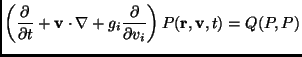
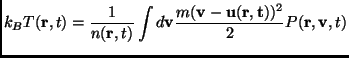
Let us quickly review the derivation of the hydrodynamic equations. The Boltzmann equation for the two models introduced in this paper (in two dimensions) reads:
where the collision integral reads, as usual:
![\begin{multline}
Q(P,P)=\sigma \int d{\bf v}_1 \int d{\bf\hat{n}} \Theta({\bf\ha...
...f r},
{\bf v}_1',t)-P({\bf r},{\bf v},t) P({\bf r},{\bf v}_1,t)]
\end{multline}](img1272.png)
Here
![]() is the unit vector along the line joining the
centers of the colliding particles at contact,
is the unit vector along the line joining the
centers of the colliding particles at contact,
![]() is the relative velocity of the colliding disks,
is the relative velocity of the colliding disks, ![]() is the
Heaviside step function,
is the
Heaviside step function, ![]() and
and
![]() are the
precollisional velocities leading after collision to velocities
are the
precollisional velocities leading after collision to velocities ![]() ,
,![]() .
.
The equation (4.11) must be completed with the boundary conditions in order to describe the microscopic evolution of the whole system.
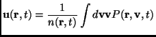
The difficulty of solving the Boltzmann equation (4.11) can
be bypassed substituting the microscopic description given by
![]() with averages given by the hydrodynamic fields: the
number density field
with averages given by the hydrodynamic fields: the
number density field
![]() , the velocity field
, the velocity field
![]() and the granular temperature field
and the granular temperature field
![]() . These
quantities are given by
. These
quantities are given by
 |
(4.12) |
 |
(4.13) |
 |
(4.14) |
These quantities, in an elastic hard spheres gas, are collisional invariants and therefore are totally conserved during the dynamics: this property guarantees that - while the fluctuations of the microscopic degrees of freedom are rapidly absorbed at the time-scale of a few collisions per particle - these few macroscopic fields slowly relax on larger time-scales. Therefore on time-scales larger than the mean free time and on space-scales larger than the mean free path (if this distinction of scales is possible) the hydrodynamic fields can be described by the hydrodynamics equations discussed ahead, where a local pseudo-equilibrium is used to close the hierarchy of the Maxwell equations for the moments. This procedure has been discussed in Chapter 2.
Multiplying the Boltzmann equation (4.11) by ![]() or
or ![]() or
or
![]() and integrating over
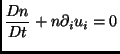
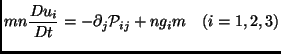
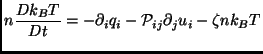
and integrating over ![]() one can derive the equations of fluid dynamics:
one can derive the equations of fluid dynamics:
where
![]() (for the sake of compactness
we use here the notation
(for the sake of compactness
we use here the notation
![]() and
and
![]() )
and
)
and
![]() is the
Lagrangian derivative, i.e.:
is the
Lagrangian derivative, i.e.:
![]() with
with
![]() the
evolution after a time
the
evolution after a time ![]() of
of ![]() under the velocity field
under the velocity field
![]() . In the above equations
. In the above equations
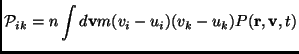 |
(4.18) |
is the stress tensor, ![]() is the volume external force (gravity
in our case),
is the volume external force (gravity
in our case),
 |
(4.19) |
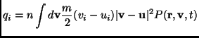
is the heat flux vector and
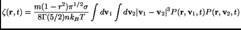 |
(4.20) |
is the cooling rate due to dissipative collisions.
The set of equations (4.16)-(4.18) become closed hydrodynamic equations
for the fields ![]() ,
, ![]() and
and ![]() when
when
![]() ,
, ![]() and
and ![]() are
expressed as functionals of these fields. This is obtained, for
example, expressing the space and time dependence of
are
expressed as functionals of these fields. This is obtained, for
example, expressing the space and time dependence of ![]() in terms of
the hydrodynamic fields and then expanding
in terms of
the hydrodynamic fields and then expanding ![]() to first order (the
so-called Navier-Stokes order) in their gradients, with the exception
of
to first order (the
so-called Navier-Stokes order) in their gradients, with the exception
of ![]() which requires an expression of
which requires an expression of ![]() to the second order of
gradients to be consistent with the other terms. With this
approximation the equations (4.16)-(4.18) include the contributions up
to the second order in the gradients of the fields.
to the second order of
gradients to be consistent with the other terms. With this
approximation the equations (4.16)-(4.18) include the contributions up
to the second order in the gradients of the fields.
We follow Brey et al. [39] and write down the hydrodynamics
for the Inclined Plane Model presented in this paper (gravity in one
direction and vibrating bottom wall, i.e.
![]() and
and
![]() ), with the following assumptions: the fields do not depend
upon
), with the following assumptions: the fields do not depend
upon ![]() (the coordinate parallel to the bottom wall),
i.e.
(the coordinate parallel to the bottom wall),
i.e.
![]() , and the system is in a steady state,
i.e.
, and the system is in a steady state,
i.e.
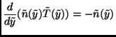
![]() . The continuity equation (4.16) then
reads
. The continuity equation (4.16) then
reads
![]() and this can be
compatible with the bottom and top walls (where
and this can be
compatible with the bottom and top walls (where ![]() ) only if
) only if
![]() , that is in the absence of macroscopic vertical flow.
The equations are written for the dimensionless fields
, that is in the absence of macroscopic vertical flow.
The equations are written for the dimensionless fields
![]() and
and
![]() , while the position
, while the position ![]() is made dimensionless using
is made dimensionless using
![]() . Finally for the pressure we put
. Finally for the pressure we put
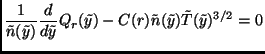
![]() . With the assumption discussed
above the equations of Brey et al read:
. With the assumption discussed
above the equations of Brey et al read:
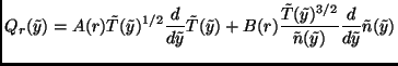
where
![]() is the granular heat flux expressed by
is the granular heat flux expressed by
In the above equations ![]() ,
, ![]() and
and ![]() are dimensionless
monotone coefficients, all with the same sign (positive), explicitly
given in the Appendix B. In particular
are dimensionless
monotone coefficients, all with the same sign (positive), explicitly
given in the Appendix B. In particular ![]() and
and ![]() , i.e. in
the elastic limit there is no dissipation and the heat transport is
due only to the temperature gradients, while when
, i.e. in
the elastic limit there is no dissipation and the heat transport is
due only to the temperature gradients, while when ![]() a term
dependent upon
a term
dependent upon
![]() appears
in
appears
in
![]() . The use of dimensionless fields eliminates the
explicit
. The use of dimensionless fields eliminates the
explicit ![]() dependence from the equations, that remains hidden
in their structure (the right hand term of equation 4.22, that is
due to the gravitational pressure gradient, disappears in the equation
for
dependence from the equations, that remains hidden
in their structure (the right hand term of equation 4.22, that is
due to the gravitational pressure gradient, disappears in the equation
for ![]() ).
).
The correct solution of Eqs. (4.22) and (4.23) has been found and published by Brey et al. [43]. We have published [15], almost contemporaneously, a wrong solution (we have done a sign error in the starting equation, obtaining wrong final equations). The error was pointed out by Eggers and also by Brey and co-workers (private communications). In the following section the correct solution is sketched.