Density correlations

We have studied (in $d=1$ and $d=2$) the arrangement of the grains inside the box and the correlations between their positions. The main feature observed in this study is the appearance of spatial clustering for inelastic gases ($r < 1$) in the colliding regime ( $\rho \gg 1$). We firstly give detailed results for $d=1$ and, after, similar measurements for $d=2$.

Figure: Density profiles in $d=1$, obtained with MD simulations with $N=L=200$ (and bins large $L_{bin}=4$). Parameters in (a) are $\tau _b=0.01$ and $r=0.99$. In (b) instead are $\tau _b=100$, $r=0.6$.

In Fig. fig_density_1d we show a profile of the density (not normalized) of the gas obtained by means of a coarse graining. The pictures are taken for two different choices of the parameters: one in the collisionless regime (and near elasticity), the other in the colliding regime. A guideline indicates the average (uniform) density. The colliding regime is characterized by fluctuations of the density very much stronger than in the collisionless regime. We call these fluctuations ``clusters''.

In Fig. fig_density_dist_1d and Fig. fig_density_dist_1d_DSMC we show the probability distribution of the ``M-cluster mass'' $m_M$ defined as the number of particles found in a box of volume $V/M$. The two figures are similar in the choices of the parameters, but the first is taken from a MD simulation, while the second from a DSMC run. These figures are important because show an impressive qualitative agreement between the two algorithms used in this work: in the collisionless regime ( $\tau_b \ll \tau_c$) the number of particle in a box is Poisson distributed, i.e.:

$$f(m_M)=\frac{\langle m_M \rangle^{m_M}}{m_M!}e^{- \langle m_M \rangle}$$ (3.14)

where $\langle m_M \rangle=N/M$ is the expected value of $m_M$. This distribution is the signature of the fact that the positions of the particles are independently distributed in the space, i.e. no correlations emerge from the dynamics in this regime. On the other side, in the colliding regime ( $\tau_b \gg \tau_c$), the distribution is very different. In both the figures it can be fitted by a curve $m_M^{-\alpha_{cl}}\exp(-c_{cl}m_M)$. This curve is the product of a negative power law with a negative exponential cut-off. In most observed situations we have measured $\alpha_{cl}>1$ and $1/c_{cl}$ slightly greater than $N/M$. The power law is the signature of self-similarity in the distribution of clusters: in the colliding regime structures emerge with no characteristic mass. The exponential cut-off is due to finite size effects ($N$ is finite and is a normalizing constraint). We stress that the agreement between MD and DSMC results is striking: these observations suggest strong correlations between grains, a fact that cannot be considered obvious in a DSMC simulation (where some correlations are artificially removed).

Figure: Distribution of cluster mass $m_M$, in $d=1$, MD. With $N=L=300$, $M=100$, one set of data with $\tau _b=0.01$ and $r=0.99$, the other with $\tau _b=100$ and $r=0.7$. The first set is fitted by a Poisson distribution with average $\overline {m}=3$, the other by a curve $m^{-1}\exp(-0.14m)$.

Figure: Distribution of cluster mass $m_M$, in $d=1$, DSMC. With $N=L=500$, $M=12000$, one set of data with $\tau _b=0.01$ and $r=0.99$, the other with $\tau _b=100$ and $r=0.5$. The first set is fitted by a Poisson distribution with average $\overline {m}=N/M \approx 0.4$, the other by a curve $m^{-1.95}\exp(-0.26m)$.

Figure: $H_M/H_M^*$ vs. $r$ in $d=1$, MD simulations, with $N=200$, $M=80$ ( $H_M^* \approx 63$), different values of $\tau _b$: $0.01$, $2$, $100$, $1000$

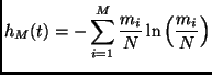
We have characterized the departure from the Poisson distribution of the cluster masses by means of an $h_M$ entropy functional which is defined as

$$h_M(t)=-\sum_{i=1}^M \frac{m_i}{N}\ln\left(\frac{m_i}{N} \right)$$ (3.15)

where the system has been divided in $M$ boxes of volume $V/M$ and the quantity $m_i$ is the number of particles in the $i$-th box. This quantity attains its maximum value $\ln M$ when the number of particle is the same, $N/M$, in every box and decreases as the density becomes more and more clusterized. As we have seen, the homogeneous regime is characterized by fluctuations of the quantity $m_i=m_M$, following the Poisson distribution of Eq. (3.15); in this case the value $h_M$ can be numerically calculated. We call this ``homogeneous'' value $h_M^*$. The value $h_M$ has the same properties of stationarity found for the kinetic energy or the dissipated energy. In Figure Fig. fig_entropy_1d_MD it is shown the quantity $H_M/H_M^*$, where $H_M=\exp(h_M)$ and $H_M^*=\exp(h_M^*)$. We observe that the departure from the collisionless regime is accompanied by a sensible decrease of the entropy of the distribution of the masses, which is a signature of the organization in dense clusters and almost empty regions. The clusters are rapidly evolving, they break and form again, so that the entropy $h_M$ is statistically stationary on large observation times (time averages).

Furtherly, to obtain more information on the kind of spatial correlations among grains, we have studied the correlation dimension (Grassberger and Procaccia [100]) $d_2$ that is defined in the following way. The cumulated particle-particle correlation function is:

$$C (t,R)=\frac{1}{N(N-1)}\sum_{i \neq j} \Theta(R-\vert{\bf x}_i(t)-{\bf x}_j(t)\vert)$$ (3.16)

After having checked that the system has reached a stationary regime, we have computed its time-average $C(R)$. In the Fig. fig_d2_1d_MD and Fig. fig_d2_1d_DSMC we show the $C(R)$ vs. $R$ for different regimes and with different algorithm. We observe a power law behavior in both colliding and collisionless regimes, and with both algorithm, MD and DSMC (this is again a surprising agreement):

$$C(R) \sim R^{d_2}$$ (3.17)

This relation defines the correlation dimension $d_2$.

In the case of homogeneous density $d_2$ is expected to be the euclidean dimension $d_2=d$. The case $d_2<d$ is a definition of fractal density. We find a homogeneous density in the collisionless regime, and fractal density in the inelastic colliding regime ( $\tau_b \gg \tau_c$ and $r < 1$). This is consistent with the power law distribution of cluster masses observed before in the same regime.

Figure: The correlation dimension $d_2$ vs $r$ for different values of $\tau _b$: $0.01$, $2$, $100$, $1000$ from top to bottom. $N=L=200$ in all the simulations, with $d=1$ MD

In Fig. fig_d2_1d we show the stationary values of $d_2$ obtained for different choices of the parameters $r$ and $\tau _b$ (keeping almost fixed $\tau_c$). We stress the fact that the DSMC algorithm imposes the absence of correlations among colliding particles: this is observed in the plot of $C(R)$ where, in the colliding regime, the slope $d_2<d$ is observed only for $R>R_0$, with $R_0 \approx r_B$ (see Fig. fig_d2_1d_MD and Fig. fig_d2_1d_DSMC) . For a discussion on the Bird radius $r_B$ we refer to Appendix A.

Figure: Density correlation function $C(R)$ vs $R$, in $d=1$, with MD simulations with $\tau _b=100$ and $r=0.99$ (bottom) and $\tau _b=100$ and $r=0.6$ (top), $N=L=200$; the measured $d_2$ takes respectively the values $1$ and $0.59$

Figure: Density correlation function $C(R)$ vs $R$, in $d=1$, with DSMC algorithm with $\tau _b=0.01$ and $r=0.99$ (bottom) and $\tau _b=100$ and $r=0.5$ (top), $N=L=2000$, $\tau _c=0.5$, $r_B=0.4$; the measured $d_2$ takes respectively the values $1$ and $0.55$

We have repeated all the analysis of the density for the system in $d=2$, using only DSMC simulations, and finding the same phenomena: homogeneous density in the case $\tau_b \ll \tau_b$ and clusterized fractal density when $\tau_b \gg \tau_c$ and $r < 1$. In Fig. fig_density_2d we propose a ``photography'' of the system with the positions of the particles, in an instant of the simulation in the clusterized regime ( $\tau_b \ll \tau_c$ and $r < 1$). In Fig. fig_density_dist_2d we show the probability distribution of cluster masses, as defined above, for the two different regimes: we observe again the Poisson distribution in the homogeneous situation and the power law (plus the finite size exponential cut-off) in the clusterized situation.

Finally, we have studied the correlation function defined in Eq. (3.17) and its power-law behavior characterized by the exponent $d_2$. The function is shown in Fig. fig_d2_2d. In Fig. fig_summary we have plotted a summary of the measurements of several quantities in $d=2$: the granular temperature, the correlation dimension $d_2$, the collision rate $\nu$ and the diffusion coefficient $D$. The diffusion coefficient is discussed in a paragraph 5.66.

Figure: Snapshot of particle distribution in $d=2$, in the clusterized regime ( $\tau _b=100$, $\tau _c=0.01$, $r=0.5$), with $N=L^2=5000$ and $r_B=0.63$

Figure: Distribution of cluster mass $m_M$, in $d=2$, DSMC simulations. With $N=L^2=10000$, $M=3200$, $\tau _c=0.05$, $r_B=0.22$, one set of data with $\tau _b=0.01$ and $r=0.99$, the other with $\tau _b=100$ and $r=0.5$. The first set is fitted by a Poisson distribution with average $\overline {m}=N/M = 3.125$, the other by a curve $m^{-0.5}\exp(-0.097m)$.

Figure: Granular temperature $T_g$, correlation dimension $d_2$, collision rate $\nu$ and diffusion coefficient $D$ vs. $r$ from DSMC simulations with $d=2$, with $N=L^2=3000$, $\tau _c=0.5$, $\tau _b=100$ and $r_B=0.5$

Figure: Density correlation function $C(R)$ vs $R$, in $d=2$, with DSMC algorithm with $\tau _b=0.01$ and $r=0.99$ (bottom) and $\tau _b=100$ and $r=0.5$ (top), $N=L^2=5000$, $\tau _c=0.5$, $r_B=0.71$; the measured $d_2$ takes respectively the values $2$ and $1.45$