Kinetic energy and dissipated kinetic energy, stationarity, thermodynamic limit

Figure: $K$ and $W$ vs $r$ in $d=1$ MD simulations, with $\tau _b$ that takes the values $0.01$, $2$, $100$, $1000$ (from top to bottom), while $\tau _c \in (0.5,5)$, $N=L=200$, $T_b=1$. The values used for $r$ are: 0, $0.2$, $0.4$, $0.6$, $0.8$ and $0.99$. Missing data points are due to the appearance of strong density fluctuations: we have discarded these points assuming that the Bird algorithm is unreliable in these situations.

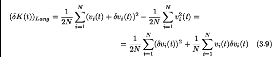
We have studied the average kinetic energy (``granular temperature'') and the average energy dissipated by the collisions of the system. These quantities are defined in the following way:

where $(\Delta K)_j$ is the kinetic energy loss during the $j_{th}$ collision occurring at time $t_j$. These quantities reach a stationary value (i.e. are ``constant'') after a transient time of the order of the longest characteristic time (which may be $\tau_c$ or $\tau _b$) and if they are time-averaged on an observation time of the same order ($\Delta t$ is taken much smaller). The stationary values of kinetic and dissipated energy are shown in Fig. fig_K+W for different choices of the restitution coefficients and of the characteristic time of the bath $\tau _b$, in $d=1$ Molecular Dynamics simulations.

In these MD simulations we can estimate the mean free time as

$$\tau_c \approx \frac{L}{2N \sqrt{T_g}}$$ (3.10)

and, as $T_g$ is observed to be almost always in the range $[T_b/10, T_b]$, using in all simulations $L/N=1$ and $T_b=1$, we expect $\tau_c \in [0.5,2]$. Our observations confirm this expectation. The analysis of Fig. fig_K+W are in agreement with the scenario proposed in the discussion of the previous paragraph. In the elastic limit $r \to 1^-$ the granular temperature tends toward the bath temperature (and the kinetic energy in collisions tends to zero). In the collisionless limit (upper curves) the granular temperature again tends toward the bath temperature and this happens for every value of $r$. In the ``colliding'' regime the system is sensible to inelasticity and the granular temperature drops under the bath temperature when $r < 1$.

Figure: K vs. W in 1d, MD. (a) $\tau _b=0.01$, (b) $\tau _b=2$, (c) $\tau _b=100$, (d) $\tau _b=1000$. The other parameters take the same values as in Fig. fig_K+W

A mean-field relation between granular temperature, bath temperature and dissipated energy in collisions can be calculated. We assume that in a small step of time of length $\Delta t$ the dissipated energy in collisions is exactly equal to energy gained from the ``bath'' (i.e. the Langevin equation) $(\Delta K(t))_{Lang}$. This is of course a rough approximation: we have already noticed that the stationarity is strictly observed only for time-averages taken on the largest time of the problem, while on shorter times the values are fluctuating (in principle these fluctuations are physical and not statistical, i.e. they should not vanish if averaged on many realizations, because they are due to the different relaxation processes that have different characteristic times) and this equality is not guaranteed.

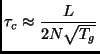
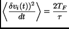
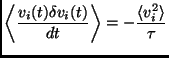
However, we try to verify this very rough relation, writing

$$\begin{multline} (\delta K(t))_{Lang} = \frac{1}{2N} \sum_{i=1}^N(v_i(t)+\delta... ...^N(\delta v_i(t))^2+ \frac{1}{N}\sum_{i=1}^Nv_i(t) \delta v_i(t) \end{multline}$$

where $\delta v_i$ is the velocity variation during a time interval $dt$ in Eq. (3.3a), from which we obtain the relations:

$$\lim_{dt \rightarrow 0} \left \langle \frac{\delta v_i(t))^2}{dt} \right \rangle = \frac{2T_F}{\tau}$$ (3.11)

$$\lim_{dt \rightarrow 0} \left \langle \frac{v_i(t) \delta v_i(t)}{dt} \right \rangle= - \frac{\langle v_i^2 \rangle}{\tau}$$ (3.12)

where the $<...>$ average is taken over different realizations of the noise.

We then insert Eqs. (3.12) and (3.13) into Eq. (3.11), assuming the equivalence among time averages, particle averages and ensemble averages, obtaining:

$$W=\frac{T_F-T_g}{\tau}$$ (3.13)

The numerical check of such relation is shown in Fig. fig_relazionewt.

This relation is fairly verified, showing that in this model fluctuations have not dramatic effects on averages and that the model is not too far from ergodicity (we have identified time averages with realization averages) and from strict stationarity (we have assumed a perfect energy balance in a time step $dt \to 0$).

Finally, we have studied the thermodynamic limit of some physical observables, using Direct Simulation Monte Carlo (see Appendix A). The quantities under study are the granular temperature $T_g$, the mean collision rate $\nu$ and the correlation dimension $d_2$. The latter quantity will be exactly defined in the next paragraph. The number of particles has been increased keeping the ratio $N/V$ fixed, in $d=1$ and $d=2$. We show the results of these simulations in Fig. fig_tl1 and Fig. fig_tl2.

The results are at odds with the same study performed on the model proposed by Du, Li and Kadanoff. There it could be obtained a stationary state with no proper thermodynamic limit. Here the existence of a proper thermodynamic limit is well verified: moreover the results in the figures show that with a few particles the observed statistical properties are compatible with that measured in bigger systems.

Figure: Thermodynamic limit in $d=1$, using DSMC algorithm (see Appendix A). Here $\tau _b=100$, $\tau _c=0.5$, $r_B=0.4$, $N/L=1$, $r=0.5$.

Figure: Thermodynamic limit in $d=2$, using DSMC algorithm (see Appendix A). Here $\tau _b=100$, $\tau _c=0.5$, $r_B=0.63$, $N/L^2=1$, $r=0.5$.