The hopping model

In this section we address the problem of the microscopic origin of the clusterization. In order to do that, we study a class of models in which the system is composed by $M$ boxes and $N$ particles assuming that the boxes have infinite connectivity (mean field hypothesis). One starts with a certain configuration and let the system evolve with an exchange dynamics in which, at each time step, one particle moves from one box to another, both boxes being chosen randomly. The probability for each single exchange is model-dependent and it will be our tuning-parameter to scan the different phenomenologies. Our goal is to understand in a quantitative way how the microscopic dynamics affects the clustering properties of the system. In particular we shall try to recover the results, obtained in the framework of the models previously introduced, for the density distributions in the clusterized and homogeneous cases (see Fig. fig_density_dist_1d, Fig. fig_density_dist_1d_DSMC, Fig. fig_density_dist_2d).

The models are defined in terms of master equations for the probability $P_m$ of having a box with $m$ particles, assigning transition rates for landing in a box with $m$ particles $W_{in} (m)$ and for leaving a box with $m$ particles $W_{out} (m)$. It must be

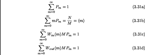
$$W_{in}(N)=W_{out}(0)=0$$ (3.31)

because no particles can be taken out of a box with 0 particles and a box with $N$ particles cannot receive any more particle. Moreover the following conditions must be satisfied:

Eq.(3.33a) is the normalization condition for $P_m$, Eq. (3.33b) is a constraint on the first moment and Eqs. (3.33c) and (3.33d) are the normalization condition for $W_{in}$ and $W_{out}$ (a particle must be taken from somewhere and put somewhere).

The general question that we want give an answer to reads: given $W_{in}$ and $W_{out}$, what is the asymptotic stationary distribution for the average number of boxes with $m$ particles, $P(m)$?

The simplest case we can consider is the one in which each single movement is independent of the state of the departing and of the landing box. In this case there is no bias in the movements and $W_{in} (m)$ and $W_{out} (m)$ do not depend upon $m$:

$$W_{in} (m) = W_{out} (m)= \frac{1}{M}$$ (3.33)

(this automatically satisfies Eqs. (3.33c) and (3.33d)), so that the general master equation reads

In the limit of $M » 1$ one can neglect the $\frac{1}{M}$ terms in the right hand side of eq. (3.35) and easily get the stationary solution ( $\frac{dP_m}{dt}=0$)

$$P_{m} = A e^{-c m}$$ (3.35)

with $A = 1- e^{-c}$ corresponding to the normalization condition $\sum_0^{\infty} P_{m} =1$ and where $c$ is a constant depending on $N$ and $M$: $c = ln(1+\frac{1}{\langle m \rangle})$ with $\langle m \rangle= \frac{N}{M}$.

This result has to be compared with the probability $f_M(m)$ in the non-clusterized cases of the previous sections. In order to do this it is necessary to recall that those results have been obtained with a small value of the number of boxes $M$. This means that one is very far from the limit $M » 1$ and this situation corresponds to a sort of coarse graining in the system in which each box (big box) is actually composed by a certain number of small boxes (whose number is such that $M » 1$). The problem can thus be formulated in the following way: given a system of $N$ particles distributed in $M_{small}$ boxes with the distribution $P_{m}$ given by eq. (3.36), what is the distribution $P^*_{m}$ for the particles in a system of $M_{big}$ boxes each one composed by $R$ ( $R=M_{small}/M_{big}$) small boxes? The resulting distribution is easily written as

$$P^*_{m}= \sum^*\prod_{i=1}^R P_{m_i}= A^R e^{-c m} F(m,R),$$ (3.36)

where $\sum^*$ indicates the sum on the $\left\{ m_1,...,m_R \right\}$ such that $\sum_{i=1}^R m_i = m$, $F(m,R)$ is the number of ways of distributing $m$ particles in $R$ boxes and it is given by:

$$F(m,R)= \binom{m+R-1}{m}$$ (3.37)

With the help of (3.38) and using the Stirling formula, the expression (3.37) becomes (for $R»N»1$)

$$\begin{multline} P_m^* = A^R e^{-cm} \frac{(m+R-1)!}{m!(R-1)!} \approx A^R e^{-c... ...prox e^{-\langle m \rangle^*} \frac{(\langle m \rangle^*)^m}{m!} \end{multline}$$

It has been used the definition of $R$, the fact that $c=\ln(1+M_{small}/N)$ and that $M_{small}/N»1$. In the last passage $\langle m \rangle^*=N/M_{big}$ has been introduced and $A^R$ has become $e^{-\langle m \rangle^*}$, as can be verified when $\langle m \rangle^{-1}=M_{small}/N»1$. It has been shown, therefore, that the coarse grained version of the solution of (3.35) is exactly the Poisson distribution found in the simulations, in the non-clusterized regime (see Fig. fig_density_dist_1d, Fig. fig_density_dist_1d_DSMC Fig. fig_density_dist_2d).

Let us consider now one case where the transition rates for the particle jumps depend on the contents of the departing and landing boxes. This corresponds to impose some sort of bias to the system that could well reproduce the situation one has in the clusterized cases due to the inelasticity. We consider in particular the following case, defined by the transition rates:

These transition rates, that satisfy the relations (3.33), have the following interpretation. The probability to land on a box containing already $m$ particles is proportional to the number of particles in order to mimic the inelastic collision with a cluster of $m$ particles. On the other hand the departure from a box containing already $m$ particles has a probability proportional to $m$ because the probability to select one particle in that particular box is proportional to $m$ (in the homogeneous case this was also true, but the fluctuation of $m$ were expected to be very small, as verified a posteriori by the Poissonian solution of the master equation).

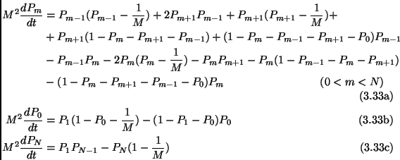
Neglecting as usual the terms of order of $\frac{1}{M}$, and after simplifications, the stationary master equations write:

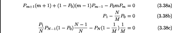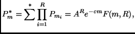
The solution in this case is given by:

with $A = \langle m \rangle (e^{c_{cl}}-1)$ and $\langle m \rangle= \frac{N}{M}$. $A$ and $c_{cl}$ are related by an implicit equation obtained imposing the condition $\sum_0^N P_{m} = 1$, that in the limit $N \rightarrow \infty$ becomes

$$1-e^{-c_{cl}}-A*\ln(1-e^{-c_{cl}})=1$$ (3.41)

In the clusterized case we expect the solution to be self-similar, in the sense that $P_m$ has the same behavior of $P_m^*$, and the coarse graining previously performed is expected not to change the solution (3.42), apart a renormalization of $\langle m \rangle$ and $c_{cl}$.

It must be noted that, as $A$ must be finite, when $N \rightarrow \infty$ (and $M$ is fixed) $c_{cl}$ has to go to zero, while $c_{cl}$ diverges when $N/M$ goes to zero. It is natural to think to $c_{cl}$ as to the inverse of the characteristic ``mass'' of a cluster, that is the typical number of particles in it. In this sense the term $\exp(-c_{cl} m)$ acts as a finite-size cut-off for the self-similar distribution $P_m \sim 1/m$, as already discussed.

The solution (3.42) is in excellent agreement with the numerical results obtained in the previous sections. In particular in the case $N=300$ $M=100$ of the MD simulations with $d=1$ one recovers the density distribution with the correct value of $c_{cl} \simeq 0.14$ (see Fig. fig_density_dist_1d).

To get the other observed behaviors of density distribution $P_m \sim e^{-c_{cl} m}/m^{\alpha_{cl}}$, it is enough to change the transition rates appearing in Eqs. (3.40a) into the following:

where $\mu$ is a normalizing constant:

$$\mu=\left( M \sum_i^N P_m m^{\alpha_{cl}} \right)^{-1}.$$ (3.43)